| Student Manual |  Faraday's law of electromagnetic induction states that an electromotive force is induced in a loop of copper wire when there is a change of magnetic flux linking the loop. According to this, the induced EMF is equal to the negative of the rate of change of flux. This principle can be tested out with an oscillating magnet that goes through a loop of wire fashioned into a solenoid. This is the case being used in the present experiment. The collected data can be used to quantitatively verify Faraday's law of electromagnetic induction. |
| Software Code | Faradays_5Missing Attachment |
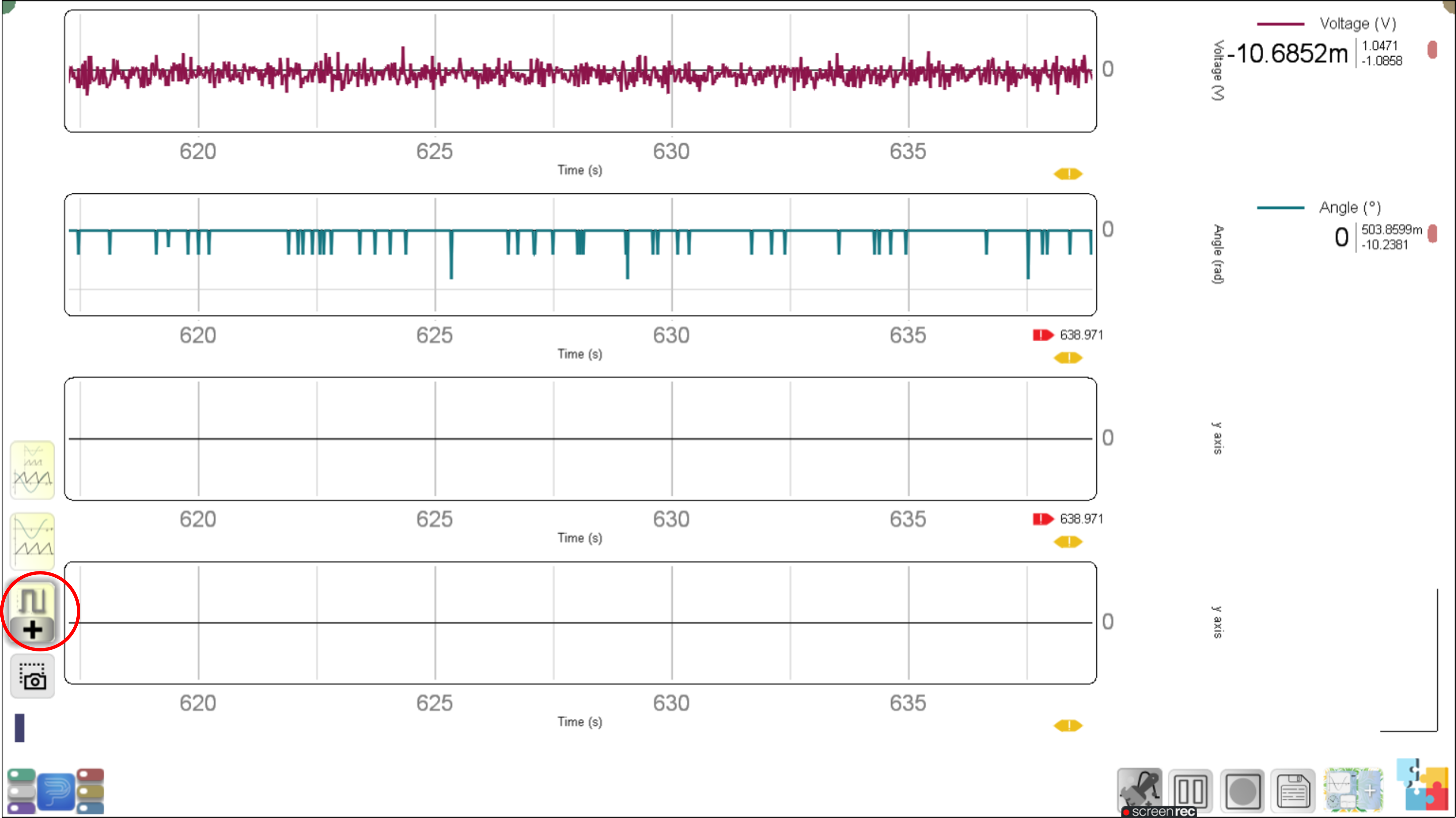
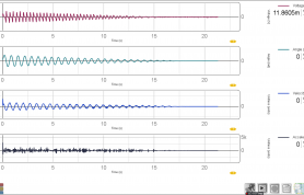
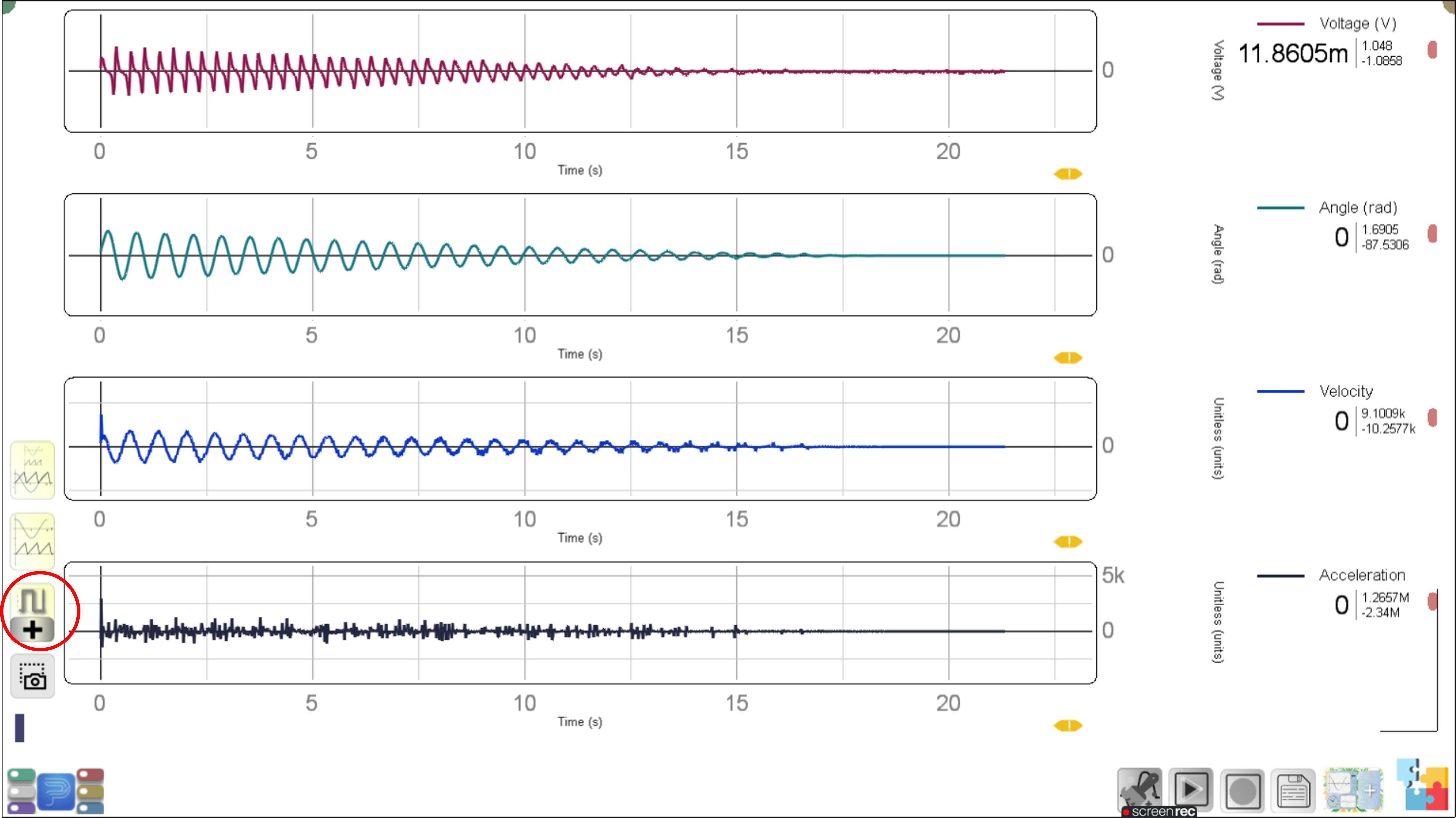
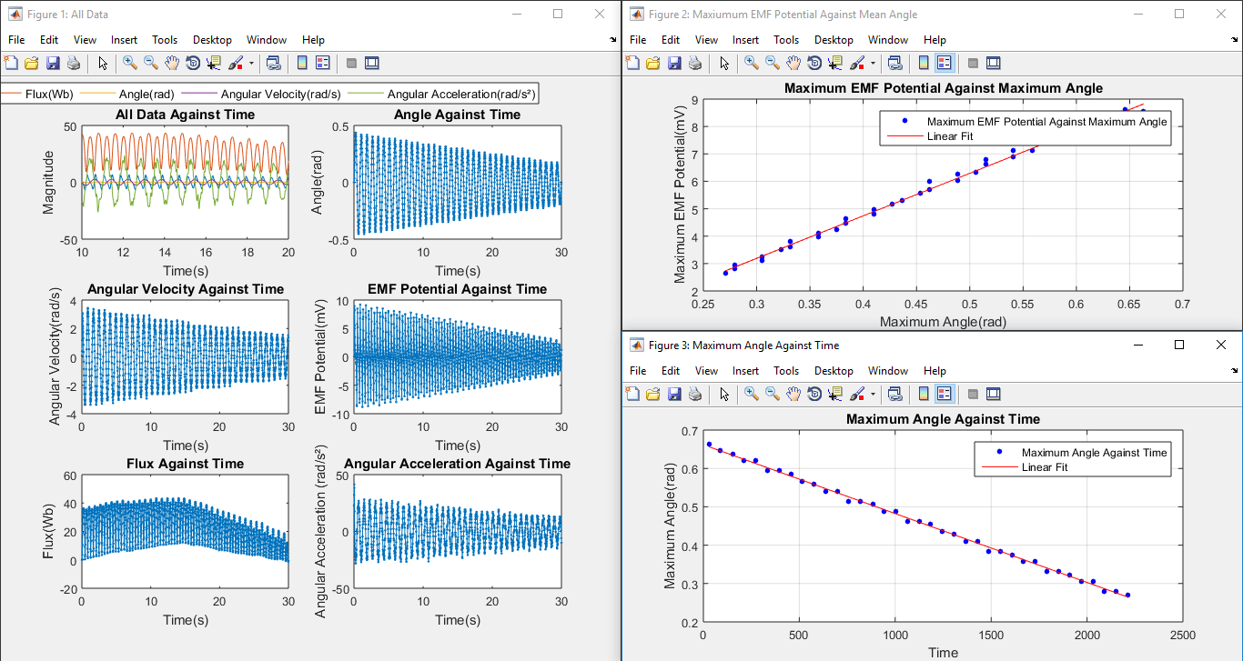
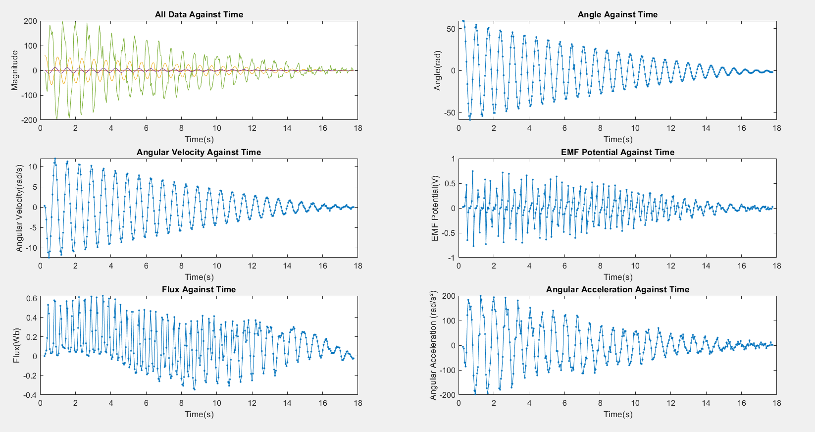
| Sample Results | Graphs of magnetic flux, EMF, angular displacement, velocity, and acceleration with time |
| Experiment Code | 1.28B |
| Version | 2022-v1 |
Further Readings and References
- Electromagnetic induction and damping: Quantitative experiments using a PC interfaceAmerican Journal of Physics, Avinash Singh, Y. N. Mohapatra, and Satyendra Kumar, .
Pictorial Procedure
-
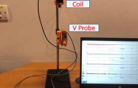
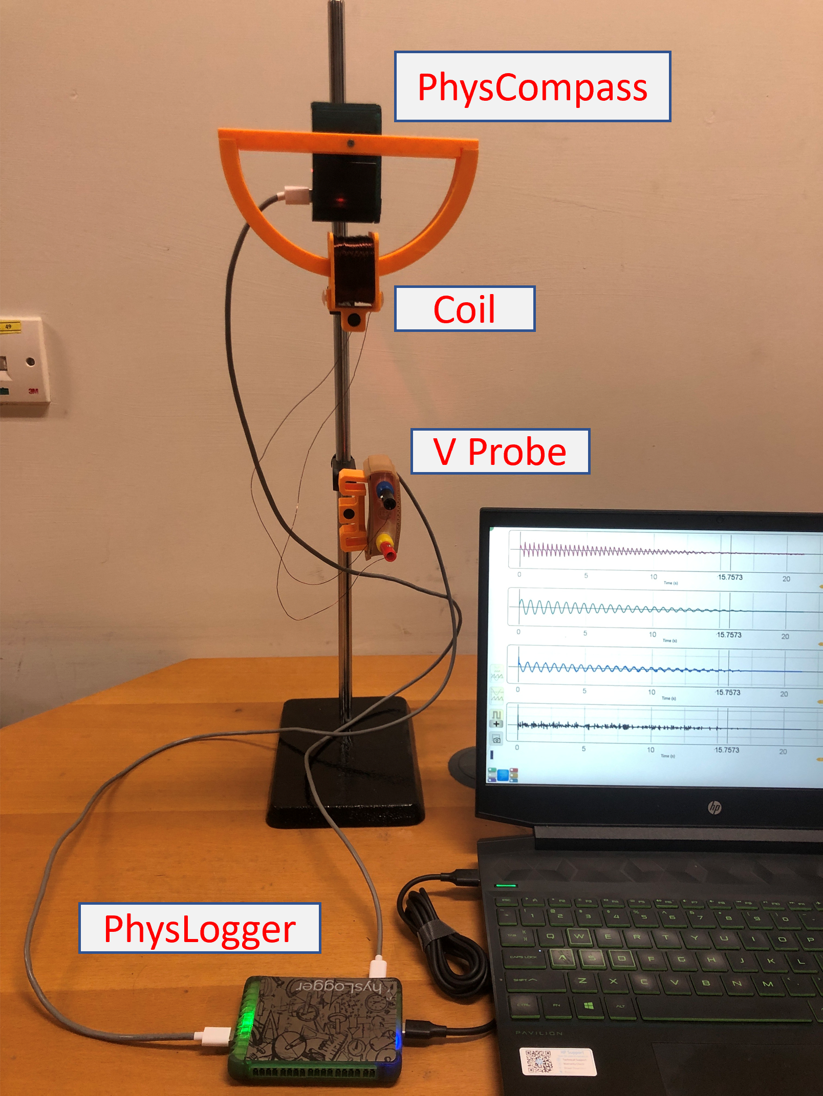
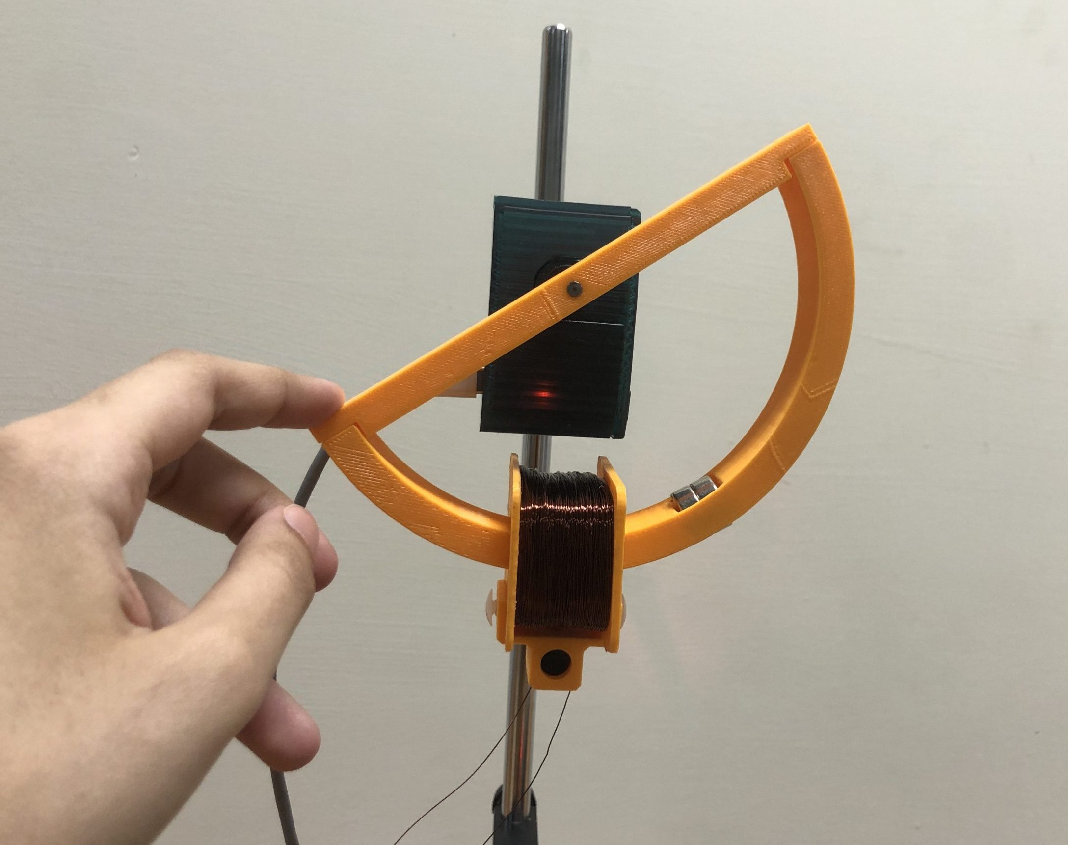
- Quantitative verification of Faraday’s law with PhysLogger Setup.
-
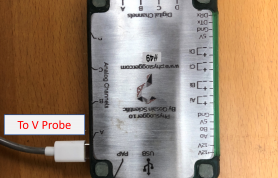
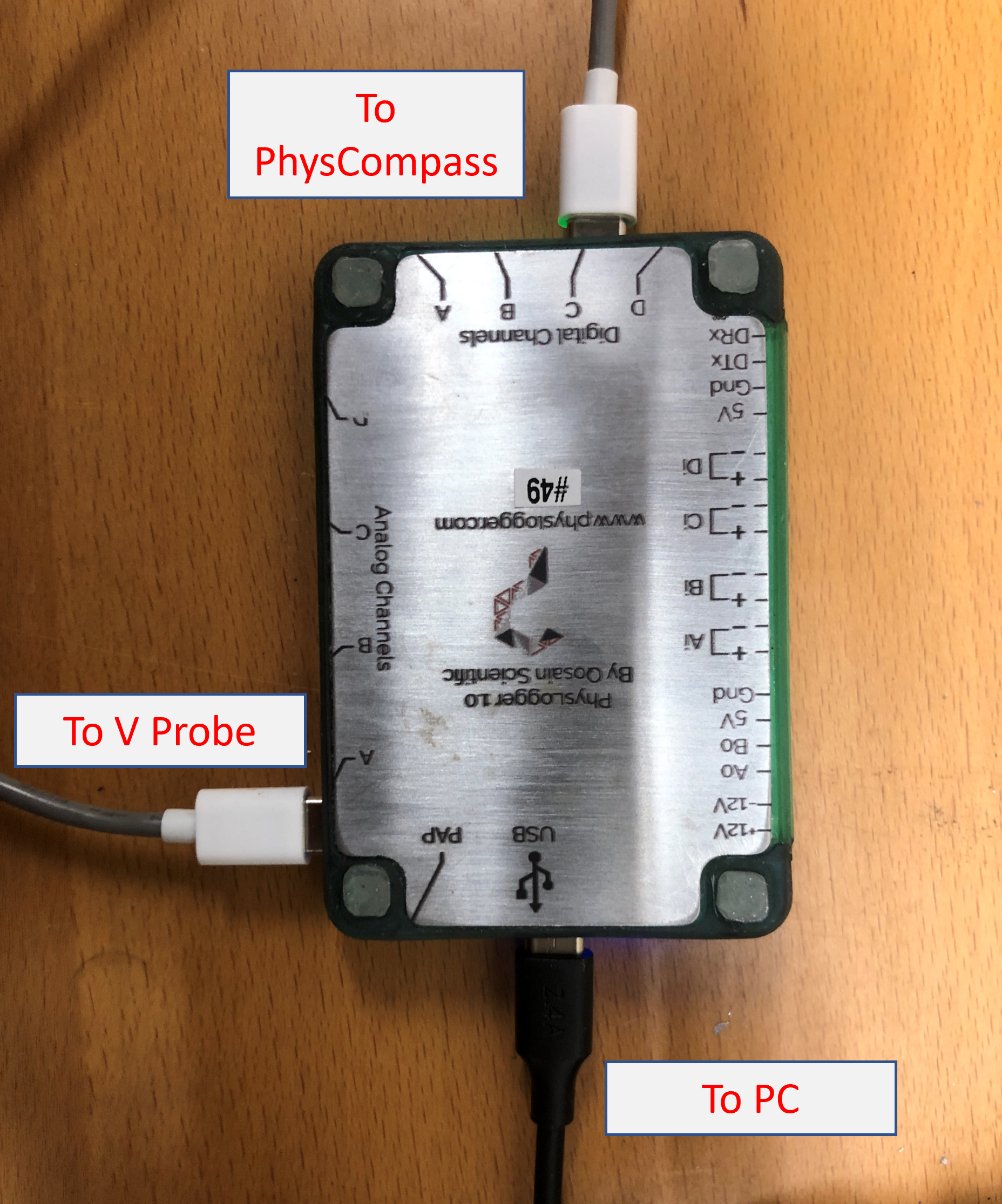
- Make all connections to PhysLogger.
-

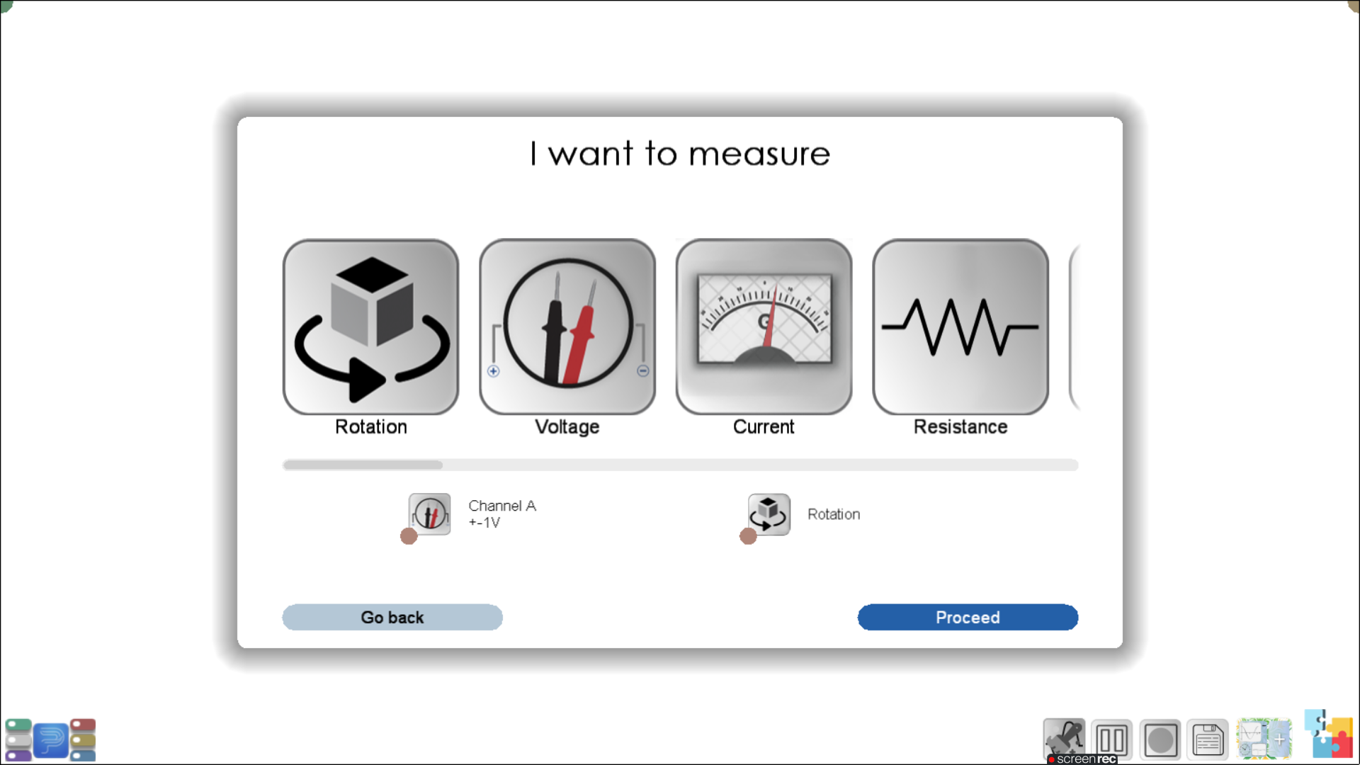
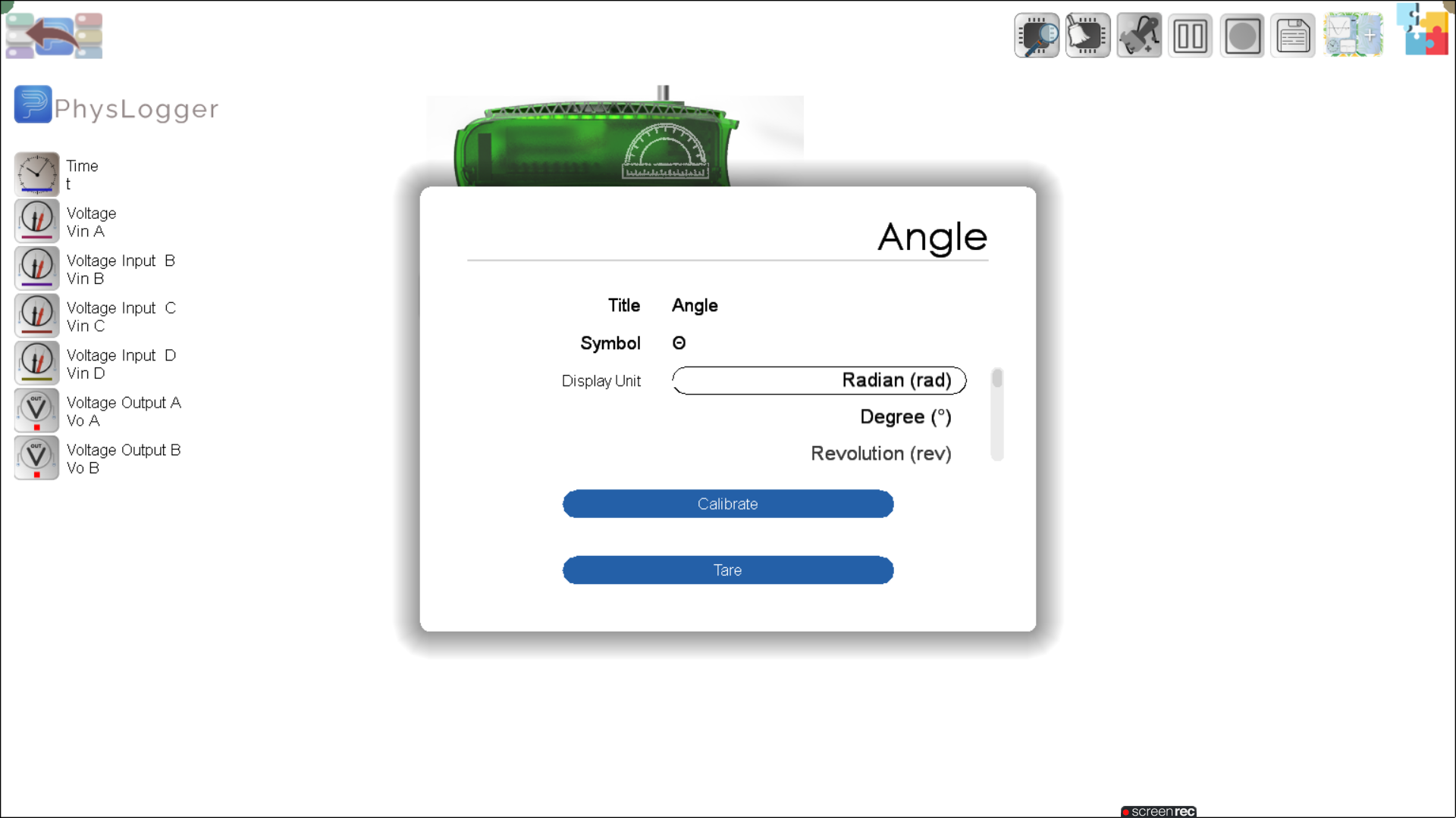
- In PhysLogger Desktop App, select Measure > Rotation and Measure > Voltage. Make a LivePlot. (PhysCompass should have been already connected to PhysLogger before starting the App).
-
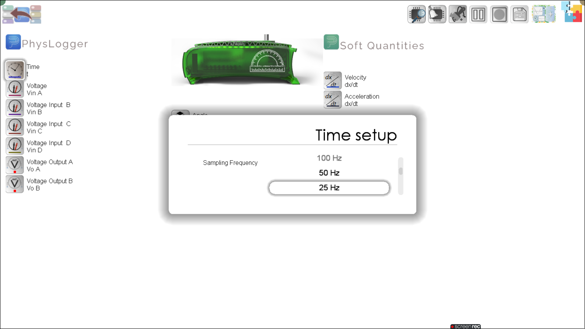
- Set sampling frequency to 50 Hz.
-
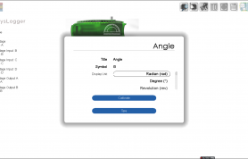
- Quantities Panel > PhysCompass > Set the units to radians. When the semicircle is stationary at its equilibrium position, Tare its readings.
-
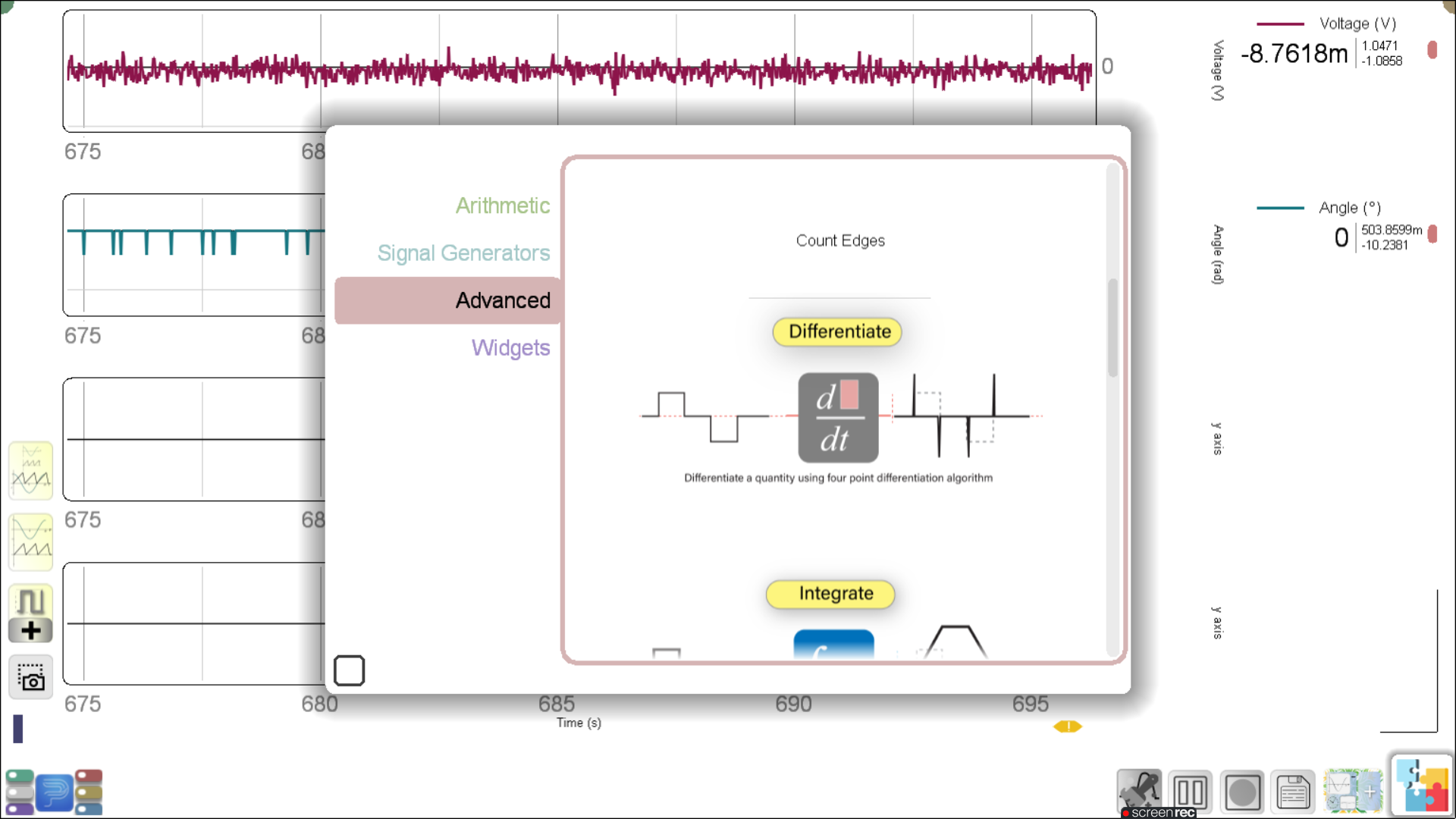
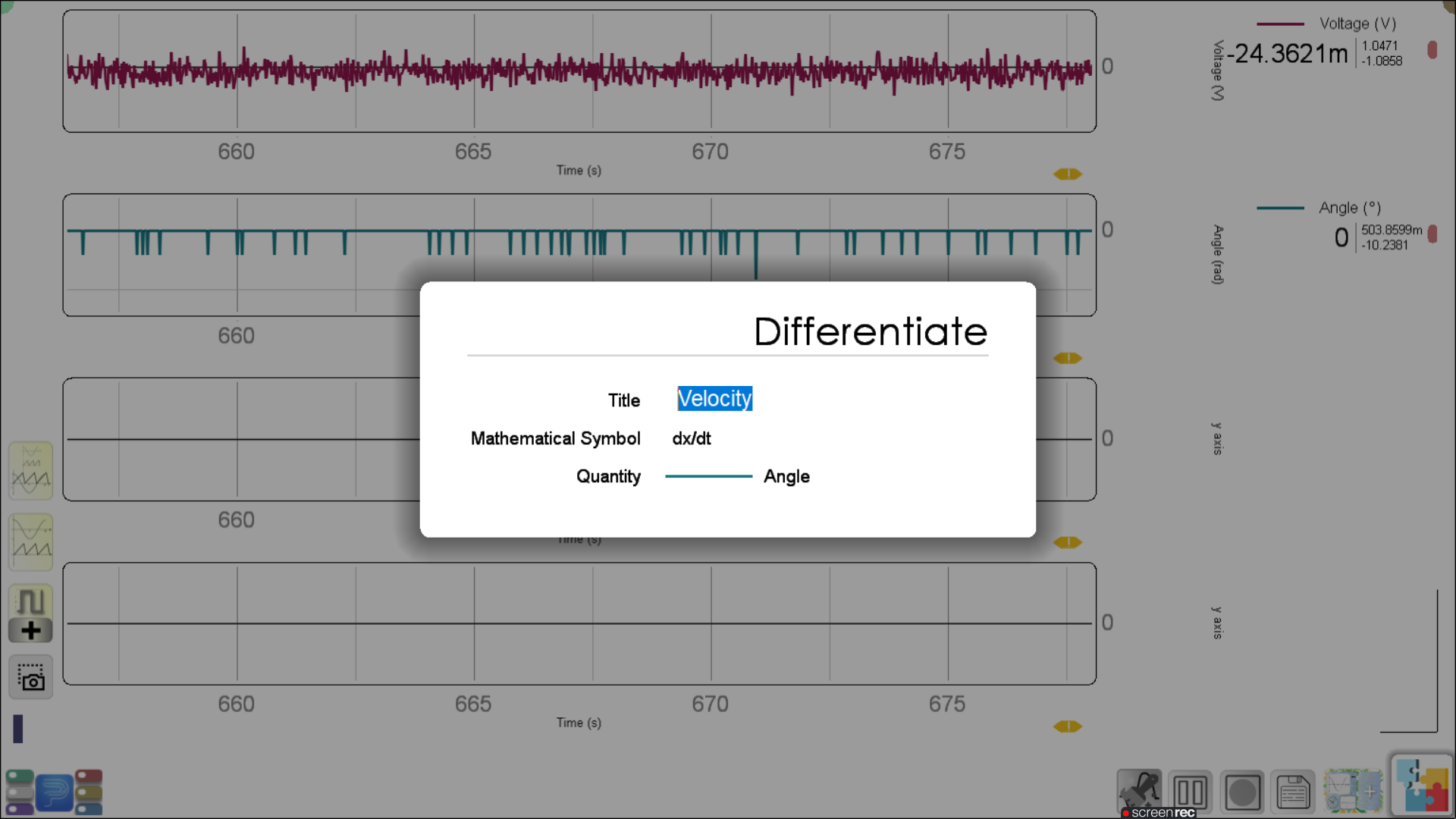
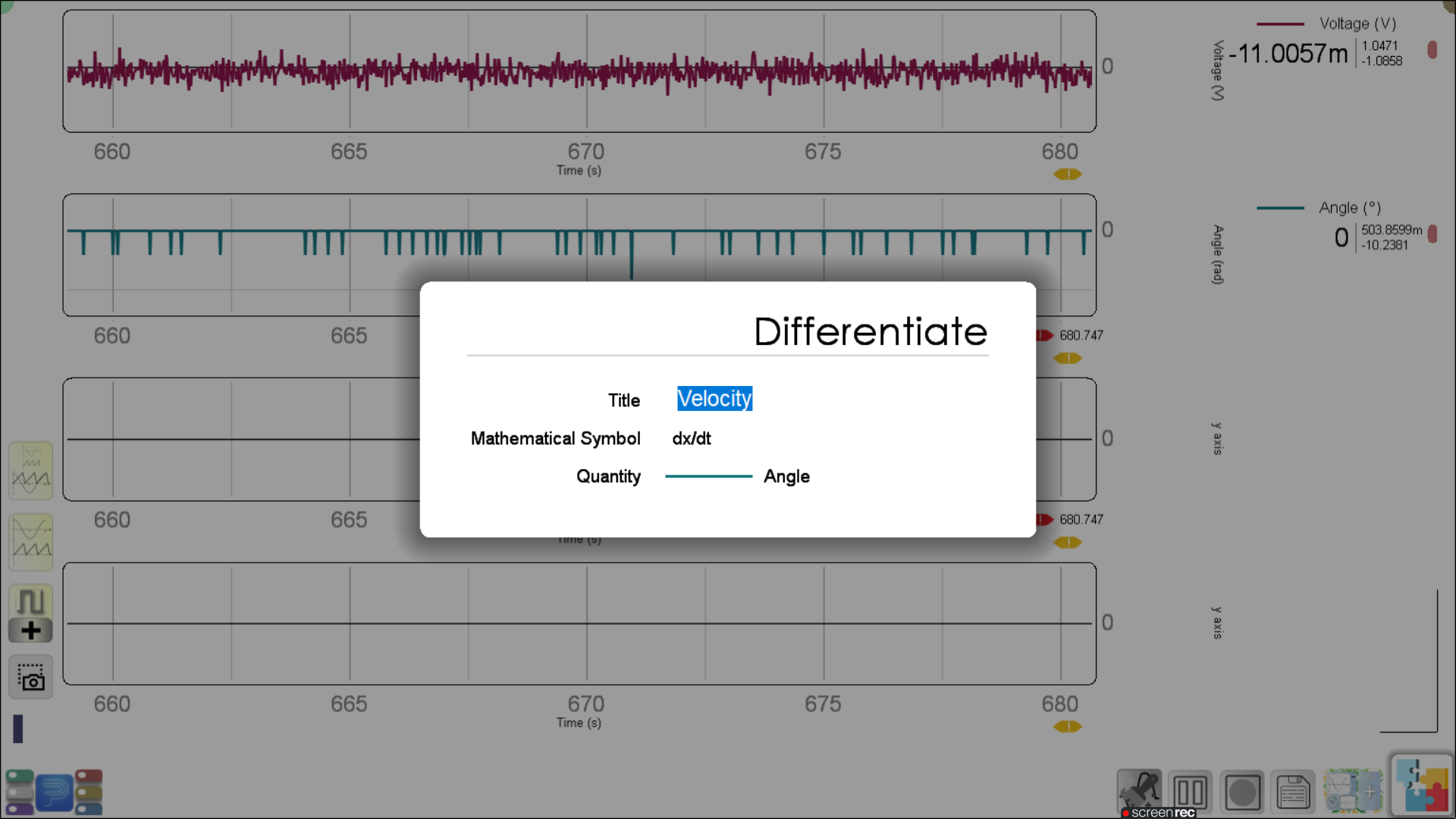
- Go to Extensions Menu > Advanced > Differentiate.
-
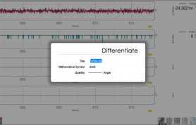
- Differentiate the angle quantity to get angular speed. (You may rename this quantity as well).
-
- Similarly, differentiate velocity to get acceleration.
-
- Add 2 more LivePlots on the same page. Drag and Drop the created differentiated quantities (Velocity and Acceleration) here.
-
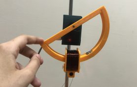
- Nudge the semicircle. (If PhysCompass readings do not oscillate perfectly, you may need to Calibrate it.)
-
- To only collect useful data, you can clear the liveplot just before releasing the semicircle.
-
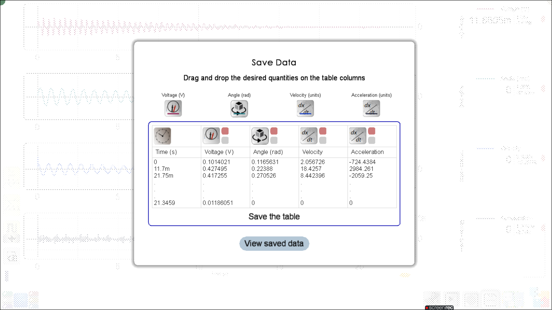
- Save all quantities > Show in Explorer. Convert the saved .csv file to .txt file. The MATLAB processing procedure is same as for 1.28.
-
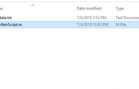
- Open ‘MainScript.m’ with MATLAB in the same folder as your data.

-
- Click on the ‘Run’ button.
-
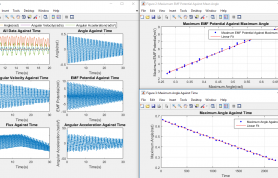
- You will receive a similar output of graphs after you have selected your data file (when prompted).